Force Fields for Materials
Machine learning force fields for studying materials has become increasingly popular. However, the large size of the physical systems associated with most materials requires some tricks to keep the amount of compute and required data sufficiently low.
In this tutorial, we will describe some of those tricks and how they can be implemented in the SchNetPack pipeline, namely:
periodic boundary conditions (PBC): PBC allow to effectively reduce the number of simulated particles to only a fraction of the actual system’s size. This is achieved by considering a relatively small simulation box, which is periodically repeated at its boundaries. In most cases, the resulting simulated periodic structure is a good approximation of the system under consideration.
cached neighbor lists: For large systems, the computation of all neighbors is expensive. In the training procedure this problem can be circumvented by utilizing neighbor list caching. This way, the neighbors must only be computed in the first epoch. In the subsequent epochs the cached neighbor lists can be loaded, which reduces the training time tremendously.
neighbor lists with skin buffer: In the scope of molecular dynamics simulations or structure relaxations, caching neighbor lists is not possible since the neighborhoods change with each integration step. Hence, it is recommended to use a neighbor list that utilizes a so-called skin buffer. The latter represents a thin layer that extends the cutoff region. It allows to reuse the calculated neighbor lists for samples with similar atomic positions. Only when at least one atom penetrates the skin buffer, the neighbor list is recalculated.
filtering out neighbors (neighbor list postprocessing): Also in the feed forward pass of the network, a large number of neighbors, and thus interactions, can result in slow inference and training. In some scenarios it is crucial to have as few operations as possible in the model to ensure fast inference. This can be achieved, e.g., by filtering out some neighbors from the neighbor list.
prediction target emphasizing: In some occasions it may be useful to exclude the properties of some atoms from the training procedure. For example you might want to focus the training on the forces of only some atoms and neglect the rest. An exemplary use case would be a model used for structure optimization where some atoms are fixed during the simulation (zero forces). Or when filtering out neighbors of certain atoms, it might be reasonable to exclude the corresponding atomic properties from the training loss.
In the following tutorial, we will first describe how the dataset must be prepared to allow for utilizing the above-mentioned tricks. Subsequently, we explain how the configs in the SchNetPack framework must be adapted for training and inference, accordingly. The dataset preparation part is based on the tutorial script “tutorial_01_preparing_data”. Please make sure you have understood the concepts introduced there, before continuing with this tutorial.
Preparing the Dataset
First we will demonstrate how to prepare the dataset to enable the use of periodic boundary conditions (pbc). “tutorial_01_preparing_data” describes how to prepare your own data for SchNetPack. For the purpose of this tutorial we will create a new dataset and add the Si\(_{16}\) diamond structure to the database. More structures can be added to the dataset by repeating the process with more datapoints in an iterative manner. In order to create the sample structure we need the atomic positions, the cell shape and the atom types. Furthermore, we want to add the properties “energy”, “forces” and “stress” to our dataset.
[1]:
import numpy as np

n_atoms = 16
positions = np.array(
    [
        [5.88321935, 2.88297608, 6.11028356],
        [3.55048572, 4.80964742, 2.77677731],
        [0.40720652, 6.73142071, 3.88666154],
        [2.73860477, 0.96144918, 0.55409947],
        [0.40533082, 4.80977264, 0.55365277],
        [2.73798189, 2.88306742, 3.88717458],
        [5.88129464, 0.96133042, 2.77731562],
        [3.54993842, 6.73126316, 6.10980443],
        [0.4072795, 2.88356071, 3.88798019],
        [2.7361945, 4.80839638, 0.55454406],
        [5.8807282, 6.732434, 6.10842469],
        [3.55049053, 0.96113024, 2.77692083],
        [5.88118878, 4.80922032, 2.7759235],
        [3.55233987, 2.8843493, 6.10940225],
        [0.4078124, 0.96031906, 0.5555672],
        [2.73802399, 6.73163254, 3.88698037],
    ]
)
cell = np.array(
    [
        [6.287023489207423, -0.00034751886075738795, -0.0008093810364881463],
        [0.00048186949720712026, 7.696440684406158, -0.001909478919115524],
        [0.0010077843421425583, -0.0033467698530393886, 6.666654324468158],
    ]
)
symbols = ["Si"] * n_atoms
energy = np.array([-10169.33552017])
forces = np.array(
    [
        [0.02808107, -0.02261815, -0.00868415],
        [-0.03619687, -0.02530285, -0.00912962],
        [-0.03512621, 0.02608594, 0.00913623],
        [0.02955523, 0.02289934, 0.0089936],
        [-0.02828359, 0.02255927, 0.00871455],
        [0.03636321, 0.02545969, 0.00911801],
        [0.0352177, -0.02613079, -0.00927739],
        [-0.02963064, -0.0227443, -0.00894253],
        [-0.03343582, 0.02324933, 0.00651742],
        [0.03955335, 0.0259127, 0.00306112],
        [0.03927719, -0.02677768, -0.00513233],
        [-0.0332425, -0.02411682, -0.00464783],
        [0.03358715, -0.02328505, -0.00626828],
        [-0.03953832, -0.02600458, -0.00316128],
        [-0.03932441, 0.02681881, 0.0048871],
        [0.03314345, 0.0239951, 0.00481536],
    ]
)
stress = np.array(
    [
        [
            [-2.08967984e-02, 1.52890659e-06, 1.44133597e-06],
            [1.52890659e-06, -6.45087059e-03, -7.26463797e-04],
            [1.44133597e-06, -7.26463797e-04, -6.04950702e-03],
        ]
    ]
)
For the purpose of filtering out certain neighbors from the neighbor list, one has to specify a list of atom indices. Between the corresponding atoms, all interactions are neglected. In our exemplary system we neglect all interactions between the atoms with index 4, 10, and 15.
[2]:
filtered_out_neighbors = np.array([4, 10, 15])
To specify the atoms, which targets should be considered in the model optimization, one must define a list of booleans, indicating considered and neglected atoms. This boolean array should be stored in the database along with other sample properties such as, e.g., energy, forces, and the array of filtered out neighbors.
For our exemplary system of 16 atoms, the array of considered atoms could be defined as follows:
[3]:
# initialize array specifying considered atoms
considered_atoms = np.ones(n_atoms, dtype=bool)

# atom 4 and atom 5 should be neglected in the model optimization
considered_atoms[[4, 10, 15]] = False
Before we can add our new data to a database for training, we will need to transform it to the correct format. The atomic structure of the new system is stored in an ase.Atoms object. In contrast to datasets without periodic boundary conditions we need to set the flag pbc=True when the ase.Atoms object is created. Both the chemical properties of the structure, as well as the settings arguments for filtering neighbors and defining the atoms to consider during training are stored in
the data dictionary corresponding to the new structure. All properties of the data dictionary need to be stored as np.ndarray. Please note, that cell dependent properties need to be unsqueezed in the first dimension.
[4]:
from ase import Atoms

atoms = Atoms(
    symbols=symbols,
    positions=positions,
    cell=cell,
    pbc=True,
)
data = dict(
    energy=np.array(energy),
    forces=np.array(forces),
    stress=np.array(stress),
    considered_atoms=considered_atoms,
    filtered_out_neighbors=filtered_out_neighbors,
)
Just as with molecular datasets, we can use the create_dataset function in order to build a new database. Since we added the considered_atoms and filtered_out_neighbors to our data dictionary, we also need to define these unitless properties in the property_unit_dict. Please note, that all structures in a dataset need to have an equal set of properties. In case some structures do not filter out any neighbors, the filtered_out_neighbors has to be set with an empty list.
[5]:
from schnetpack.data import create_dataset, AtomsDataFormat

db_path = "./si16.db"
new_dataset = create_dataset(
    datapath=db_path,
    format=AtomsDataFormat.ASE,
    distance_unit="Ang",
    property_unit_dict=dict(
        energy="eV",
        forces="eV/Ang",
        stress="eV/Ang/Ang/Ang",
        considered_atoms="",
        filtered_out_neighbors="",
    ),
)
We can now add our datapoint to the new dataset:
[6]:
new_dataset.add_systems(
    property_list=[data],
    atoms_list=[atoms],
)
It is important that the entries in the dataset have the appropriate dimensions. To this end we print out the shapes of the tensors in our first data point.
[7]:
for key, value in new_dataset[0].items():
    print(key, value.shape)
_idx torch.Size([1])
energy torch.Size([1])
forces torch.Size([16, 3])
stress torch.Size([1, 3, 3])
considered_atoms torch.Size([16])
filtered_out_neighbors torch.Size([3])
_n_atoms torch.Size([1])
_atomic_numbers torch.Size([16])
_positions torch.Size([16, 3])
_cell torch.Size([1, 3, 3])
_pbc torch.Size([3])
Let`s remove the database again, because it will no longer be needed during this tutorial:
[8]:
import os

os.remove(db_path)
Adapting the Configs in the SchNetPack Framework
Now we will cover, how to adapt config files to enable the use of the above mentioned tricks in SchNetPack’s training procedure and MD framework
SchNetPack Training
Provided that appropriate neighbor list providers (ASE or MatScipy) are used, this is sufficient for using pbc in the SchNet/PaiNN framework.
The neighbor list caching is implemented in the schnetpack transform schnetpack.transform.CachedNeighborList. SchNetPack provides a transform for caching neighbor lists. It basically functions as a wrapper around a common neighbor lists. For further information regarding the CachedNeighborList please refer to the corresponding docstring in the SchNetPack code.
Neighbors can be filtered out by using the neighbor list postprocessing transform schnetpack.transform.FilterNeighbors.
To ensure that only the specified atoms are considered for the training on a certain property, the respective ModelOutput object has to be adapted. This is achieved by using so-called constraints. Each ModelOutput object takes a list of constraints. For a precise explanation on how to use schnetpack.task.ModelOutput please refer to notebook “tutorial_02_qm9”. To specify the selection of atoms for training we use the constraint transform schnetpack.task.ConsiderOnlySelectedAtoms. It has
the attribute selection_name, which should be a string linking to the array of specified atoms stored in the database.
For adding the stress property to the learning task, we need to make some modifications to configs. First of all, the Forces output module needs a stress key and the flag calc_stress=True needs to be set. Then we also need to add the stress predictions to the outputs, so it can be included in the loss function. Since the absolute values of the stress tensors are generally significantly lower than for energy and forces we need to select a comparably high loss_weight. Finally, we
need to add the Strain module to the input modules before pairwise distances.
The following is an example of an experiment config file that utilizes the above-mentioned tricks:
# @package _global_

defaults:
  - override /model: nnp

run.path: runs

globals:
  cutoff: 5.
  lr: 5e-4
  energy_key: energy
  forces_key: forces
  stress_key: stress
data:
  distance_unit: Ang
  property_units:
    energy: eV
    forces: eV/Ang
    stress: eV/Ang/Ang/Ang
  transforms:
    - _target_: schnetpack.transform.RemoveOffsets
      property: energy
      remove_mean: True
    - _target_: schnetpack.transform.CachedNeighborList
      cache_path: ${run.work_dir}/cache
      keep_cache: False
      neighbor_list:
        _target_: schnetpack.transform.MatScipyNeighborList
        cutoff: ${globals.cutoff}
      nbh_transforms:
        - _target_: schnetpack.transform.FilterNeighbors
          selection_name: filtered_out_neighbors
    - _target_: schnetpack.transform.CastTo32
  test_transforms:
    - _target_: schnetpack.transform.RemoveOffsets
      property: energy
      remove_mean: True
    - _target_: schnetpack.transform.MatScipyNeighborList
      cutoff: ${globals.cutoff}
    - _target_: schnetpack.transform.FilterNeighbors
      selection_name: filtered_out_neighbors
    - _target_: schnetpack.transform.CastTo32

model:
  input_modules:
    - _target_: schnetpack.atomistic.Strain
    - _target_: schnetpack.atomistic.PairwiseDistances
  output_modules:
    - _target_: schnetpack.atomistic.Atomwise
      output_key: ${globals.energy_key}
      n_in: ${model.representation.n_atom_basis}
      aggregation_mode: sum
    - _target_: schnetpack.atomistic.Forces
      energy_key: ${globals.energy_key}
      force_key: ${globals.forces_key}
      stress_key: ${globals.stress_key}
      calc_stress: True
  postprocessors:
    - _target_: schnetpack.transform.CastTo64
    - _target_: schnetpack.transform.AddOffsets
      property: energy
      add_mean: True

task:
  optimizer_cls: torch.optim.AdamW
  optimizer_args:
    lr: ${globals.lr}
    weight_decay: 0.01
  outputs:
    - _target_: schnetpack.task.ModelOutput
      name: ${globals.energy_key}
      loss_fn:
        _target_: torch.nn.MSELoss
      metrics:
        mae:
          _target_: torchmetrics.regression.MeanAbsoluteError
        mse:
          _target_: torchmetrics.regression.MeanSquaredError
      loss_weight: 0.0
    - _target_: schnetpack.task.ModelOutput
      name: ${globals.forces_key}
      constraints:
        - _target_: schnetpack.task.ConsiderOnlySelectedAtoms
          selection_name: considered_atoms
      loss_fn:
        _target_: torch.nn.MSELoss
      metrics:
        mae:
          _target_: torchmetrics.regression.MeanAbsoluteError
        mse:
          _target_: torchmetrics.regression.MeanSquaredError
      loss_weight: 1.0
    - _target_: schnetpack.task.ModelOutput
      name: ${globals.stress}
      loss_fn:
        _target_: torch.nn.MSELoss
      metrics:
        mae:
          _target_: torchmetrics.regression.MeanAbsoluteError
        mse:
          _target_: torchmetrics.regression.MeanSquaredError
      loss_weight: 100.
SchNetPack MD and Structure Relaxation
In the framework of MD simulations and structure relaxations it is preferable to utilize neighbor lists with skin buffers. The corresponding class in SchNetPack is called schnetpack.transform.SkinNeighborList. It takes as an argument a conventional neighbor list class such as, e.g., ASENeighborList, post-processing transforms for manipulating the neighbor lists and the cutoff skin which defines the size of the skin buffer around the actual cutoff region. Please choose a sufficiently large
cutoff skin value to ensure that between two subsequent samples no atom can penetrate through the skin into the cutoff sphere of another atom if it is not in the neighbor list of that atom.
_target_: schnetpack.md.calculators.SchNetPackCalculator
required_properties:
  - energy
  - forces
model: ???
force_label: forces
energy_units: kcal / mol
position_units: Angstrom
energy_label: energy
stress_label: null
script_model: false

defaults:
  - neighbor_list:
    _target_: schnetpack.transform.SkinNeighborList
    cutoff_skin: 2.0
    neighbor_list:
      _target_: schnetpack.transform.ASENeighborList
      cutoff: 5.0
    nbh_transforms:
      - _target_: schnetpack.transform.FilteredNeighbors
        selection_name: filtered_out_neighbors
Structure Optimization
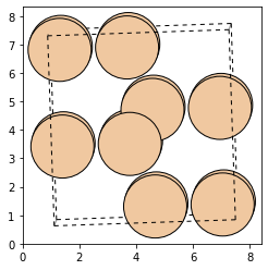
In order demonstrate the structure optimization with a trained model, we use our optimized atoms structure and add noise to the positions. Subsequently, we use a trained model and run the optimization on the noisy structure. This should return the local optimum again. Let`s first take a look our sample structure:
[9]:
from ase.visualize.plot import plot_atoms

plot_atoms(atoms, rotation=("90x,0y,0z"))
[9]:
<Axes: >
Now we create the noisy structure by adding noise to the positions and the cell:
[10]:
noise = 0.7
atms_noise = atoms.copy()
atms_noise.positions += (np.random.random(atms_noise.positions.shape) - 0.5) * noise
atms_noise.cell += (np.random.random(atms_noise.cell.shape) - 0.5) * noise
plot_atoms(atms_noise, rotation=("90x,0y,0z"))
[10]:
<Axes: >
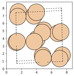
As we can see, the new structure is visibly deformed. With the use of a trained model, the structure optimizer from ase and the schnetpack.interfaces.ase_interface.SpkCalculator we will now denoise our structure. The model has been trained for the purpose of this tutorial on a small dataset of 500 Si16 structures form different local minima. It uses a SO3Net representation with 64 features and 2 interaction layers. Since we also added noise to the cell, we will wrap the atoms object
in an ExpCellFilter. Now let`s run the optimization:
[11]:
import schnetpack as spk
from schnetpack.transform import ASENeighborList
from schnetpack.interfaces.ase_interface import SpkCalculator
from ase.optimize.lbfgs import LBFGS
from ase.constraints import ExpCellFilter

# Load model
model_path = "../../tests/testdata/si16.model"

# Get calculator and optimizer
atms_noise.calc = SpkCalculator(
    model=model_path,
    stress_key="stress",
    neighbor_list=ASENeighborList(cutoff=7.0),
    energy_unit="eV",
)
optimizer = LBFGS(ExpCellFilter(atms_noise))

# run optimization
optimizer.run()
/home/docs/checkouts/readthedocs.org/user_builds/schnetpack/envs/latest/lib/python3.12/site-packages/schnetpack/utils/compatibility.py:31: UserWarning: Model was saved without version information. Conversion to current version may fail.
  warnings.warn(
/tmp/ipykernel_2106/1364696670.py:17: FutureWarning: Import ExpCellFilter from ase.filters
  optimizer = LBFGS(ExpCellFilter(atms_noise))
       Step     Time          Energy          fmax
LBFGS:    0 15:09:53   -10156.692613       11.349278
LBFGS:    1 15:09:53   -10159.390783       24.651014
LBFGS:    2 15:09:54   -10158.157812       29.762627
LBFGS:    3 15:09:54   -10162.996304       15.320600
LBFGS:    4 15:09:54   -10162.399117       25.687670
LBFGS:    5 15:09:54   -10165.639401       11.943863
LBFGS:    6 15:09:54   -10165.580474       19.901173
LBFGS:    7 15:09:55   -10167.034162        4.286935
LBFGS:    8 15:09:55   -10167.444310        4.942165
LBFGS:    9 15:09:55   -10168.008481        8.064139
LBFGS:   10 15:09:55   -10168.221655        2.960223
LBFGS:   11 15:09:56   -10168.332117        4.077005
LBFGS:   12 15:09:56   -10168.468864        2.024409
LBFGS:   13 15:09:56   -10168.580944        4.446587
LBFGS:   14 15:09:56   -10168.659301        3.778034
LBFGS:   15 15:09:56   -10168.735569        0.809232
LBFGS:   16 15:09:57   -10168.813206        1.270481
LBFGS:   17 15:09:57   -10168.903710        2.240006
LBFGS:   18 15:09:57   -10168.953359        1.257695
LBFGS:   19 15:09:57   -10168.973342        0.326535
LBFGS:   20 15:09:57   -10168.982766        0.420948
LBFGS:   21 15:09:58   -10168.990137        0.566808
LBFGS:   22 15:09:58   -10168.994049        0.306669
LBFGS:   23 15:09:58   -10168.995808        0.106649
LBFGS:   24 15:09:58   -10168.997096        0.199490
LBFGS:   25 15:09:59   -10168.998328        0.256160
LBFGS:   26 15:09:59   -10168.999175        0.147251
LBFGS:   27 15:09:59   -10168.999658        0.056075
LBFGS:   28 15:09:59   -10168.999996        0.094645
LBFGS:   29 15:09:59   -10169.000271        0.112191
LBFGS:   30 15:10:00   -10169.000442        0.058259
LBFGS:   31 15:10:00   -10169.000539        0.020937
[11]:
np.True_
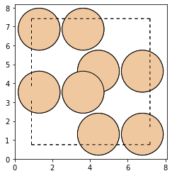
As we can see, the structure optimization has removed the noise, and we obtain our stable structure again (the stable structure may be rotated by some degree):
[12]:
plot_atoms(atms_noise, rotation=("90x,0y,0z"))
[12]:
<Axes: >